

The hidden bottlenecks between GPU capacity, inference scheduling, memory, and the experience your customers actually receive.
View the static cover. Each diagram also includes a full-size static alternative.

XTechStacks Weekly | November 14, 2026
Imagine a SaaS company that has just launched an AI-powered customer support assistant.
This edition focuses on teams operating self-hosted models or dedicated inference infrastructure. Teams using managed model APIs can apply the workload and latency diagnostics, but typically cannot tune the provider's GPU scheduling or KV-cache allocation.
The engineering team has deployed an open-weight language model on GPU infrastructure.
The initial results look promising.
During testing, responses arrive quickly. The application feels responsive, and the GPU monitoring dashboard indicates plenty of available capacity.
Then the product reaches more customers.
Support teams begin reporting that some questions take several seconds before the first word appears.
Other responses start quickly but generate text painfully slowly.
The infrastructure team checks the GPU metrics.
Average GPU utilization is only around 40%.
The assumption seems obvious.
We have capacity available. Why are customers still waiting?
The team considers adding more GPUs.
But that may be the wrong first move.
The actual bottleneck could involve request scheduling, prompt processing, GPU memory, token generation, or something outside the GPU entirely.
The example is hypothetical, but the underlying engineering problem is well established.
AI inference performance cannot be understood from GPU utilization alone.
And as enterprises move from experimenting with AI models to serving hundreds or thousands of users, this distinction becomes a serious architecture and business concern.
LLM inference performance: why GPU capacity is not enough
We are accustomed to measuring application infrastructure through CPU utilization, memory consumption, request throughput, error rates, and response times.
These metrics remain useful.
But large language models introduce performance characteristics that differ from conventional web applications.
A typical application request may execute a predictable sequence of database queries and business logic.
An LLM inference request has additional dimensions.
One customer may submit a 200-token question and request a short answer.
Another may send a 15,000-token document and ask for a detailed analysis.
A third may be part of a workflow that repeatedly sends growing conversation histories.
All three requests may use the same model endpoint.
Yet their computational and memory requirements can be dramatically different.
The number of concurrent users matters.
The length of their prompts matters.
The number of output tokens matters.
Cache reuse matters.
The scheduling decisions of the inference engine matter.
And the GPU memory available for active requests matters.
Two AI applications using the same GPU and the same model can have very different capacity limits.
That is why selecting AI infrastructure based primarily on GPU specifications or a benchmark's maximum tokens per second can lead to disappointing production results.
The two workloads hiding inside every LLM response
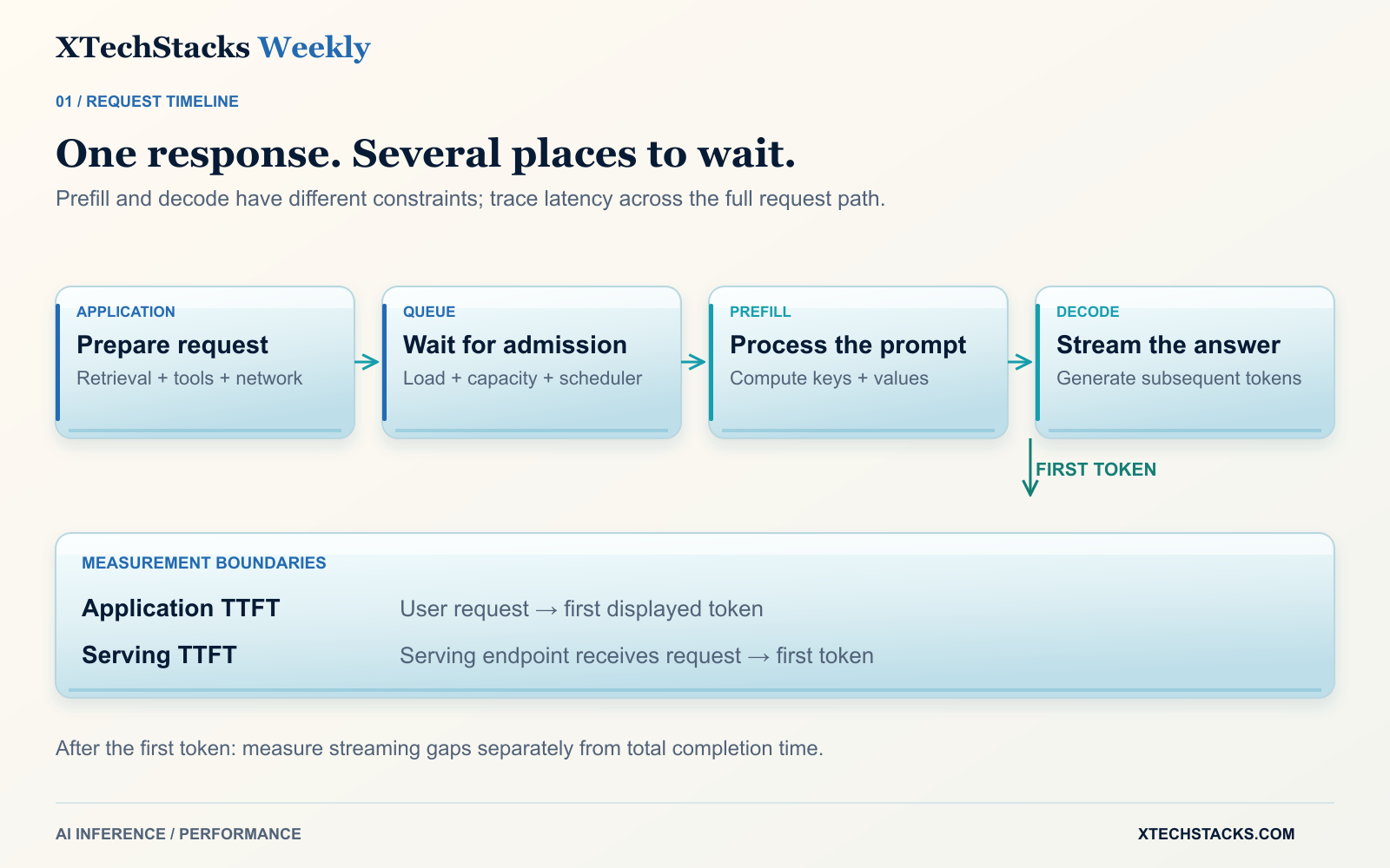
To understand why inference slows down, we need to understand what happens when a model generates a response.
Most autoregressive LLM inference involves two major phases.
First: Prefill — understanding the incoming context
During prefill, the model processes the input prompt. For conventional transformer models, it builds attention keys and values that can be reused during generation.
These are stored in the key-value cache, or KV cache.
Prefill can take advantage of parallel GPU computation.
But longer prompts generally require more work, and the attention computation can become expensive as context length increases.
For example, a customer-support assistant might initially receive a short question.
Later, the company adds retrieval-augmented generation.
Now the same question arrives with several retrieved documents, conversation history, instructions, and contextual information.
The model may be unchanged.
The GPU may be unchanged.
But the prefill workload has grown significantly.
One visible consequence is an increase in Time to First Token (TTFT)—how long the user waits before the model begins producing its response.
Second: Decode — generating the answer
Once the model has processed the prompt, it generates new tokens sequentially.
Each subsequent token depends on the preceding context.
This phase behaves differently from prefill.
Decode often becomes constrained by memory bandwidth and the movement of model weights and cached attention data, particularly at smaller batch sizes.
The GPU's arithmetic units may not be continuously saturated, even while memory movement or scheduling limits performance.
The user experiences this as slow text generation.
A response may begin quickly but then appear one word or token at a time with noticeable delays.
The gaps between streamed tokens are described by Inter-Token Latency (ITL). Some tools also report time per output token (TPOT), a per-request average. These measures are related but not interchangeable; use the benchmark tool's definitions consistently.
The distinction matters because improving prefill performance does not automatically improve decode performance.
And optimizing decode can sometimes make time to the first token worse.
The important takeaway
Slow first token? Investigate queuing and prefill.
Slow generation after the first token? Investigate decode, memory bandwidth, batching, and cache pressure.
These are diagnostic starting points, not universal diagnoses.
A complete investigation must also consider networking, tokenization, application processing, and other dependencies.
Why the GPU utilization dashboard can mislead you
Suppose your infrastructure dashboard shows 40% average GPU utilization.
What does that tell you?
First, check which metric the dashboard displays. NVIDIA's conventional GPU-utilization measure reports the share of sampled time during which at least one kernel was executing. It does not directly measure the fraction of peak arithmetic throughput being used.
A 40% average can also hide busy intervals or imbalance across GPUs. Memory bandwidth, compute activity, memory allocation, and user latency need separate measurements.
Metric definition: NVIDIA NVML
It does not necessarily reveal whether your inference service can meet user-facing latency requirements.
Several different problems can exist behind the same number.
Scenario A: The GPU is waiting for work
Requests may be delayed in an upstream API, application gateway, tokenizer, or CPU-side processing step.
The GPU is not the bottleneck.
Adding another GPU may simply increase idle capacity.
Scenario B: The GPU is limited by memory behavior
Decode may involve repeated access to model weights and KV-cache data.
Compute efficiency can be limited by memory bandwidth or the serving configuration. This is a separate observation from a low kernel-active-time percentage; a memory-bound kernel can still register as an active GPU.
Scenario C: The inference scheduler is creating contention
Long prompts may compete with active generation requests.
Depending on the scheduler, new prefill work can interrupt or delay token generation for requests already in progress.
The average utilization number cannot tell you which users are experiencing those delays.
Scenario D: The service lacks enough KV-cache capacity
A model's weights may fit comfortably into GPU memory.
But the serving engine also needs memory for active request state, temporary tensors, and KV-cache blocks.
As concurrency and context lengths increase, available KV-cache capacity may become the limiting resource.
Requests may queue, and some configurations may trigger preemption or recomputation.
The crucial distinction is between how busy the hardware looks and how much useful work the system delivers within an acceptable response time.
The metric I would put next to GPU utilization: Goodput
Most inference benchmarks report throughput.
For example:
This deployment can generate X output tokens per second.
That is useful.
But consider two configurations.
Configuration A
The server produces a large number of tokens per second, but many users experience unacceptable delays.
Configuration B
The server produces fewer total tokens, but substantially more user requests finish within the application's response-time targets.
Which configuration is better?
For an interactive enterprise application, Configuration B may provide more useful capacity.
This is where goodput becomes valuable.
Goodput measures the rate of successfully completed requests that satisfy defined service-level objectives, such as latency thresholds.
For this article, request goodput means successful requests meeting all specified latency objectives divided by the measurement duration. Set those objectives before comparing configurations.
It helps separate total completed throughput from service capacity that meets the latency contract. It does not establish that the answers are correct or safe: maintain separate quality checks and compare configurations at an acceptable quality level.
The important measurements include:
| Metric | What it tells you |
|---|---|
| Time to First Token (TTFT) | How long users wait before generation starts |
| Inter-Token Latency (ITL) | How smoothly streamed text is generated |
| End-to-end latency | How long the complete response takes |
| Request throughput | Number of completed requests per second |
| Output-token throughput | Total generation capacity |
| KV-cache utilization | How much allocated cache capacity is occupied |
| Queue time and request backlog | Whether requests are waiting for serving capacity |
| Goodput | How many requests complete within defined latency requirements |
Measure from explicit boundaries: application-level TTFT should run from the user request to the first displayed token, while a serving-engine metric starts inside that service. Retrieval, tool calls, gateways and network buffering can contribute to the difference.
For service targets, I would look at p95 and p99 behavior rather than relying only on averages. Keep per-token distributions separate from per-request averages, and report the observation count and test duration.
The p95 value describes a level at or below which approximately 95% of measured observations fall.
That is important because a system can have an excellent average latency while a meaningful share of customers experience poor performance.
And the targets should vary by workload.
A customer-facing conversational assistant might require rapid first-token response.
A background document analysis job may tolerate considerably longer latency in exchange for higher throughput or lower infrastructure cost.
The right optimization target is not maximum GPU utilization. It is dependable service performance at an economically acceptable cost.
What current research tells us
In September 2026, NVIDIA published guidance on GPU sizing for AI inference.
Its central recommendation was to begin with workload characteristics—model selection, daily active users, concurrency, input and output lengths, cache hit rates, and latency targets—rather than simply selecting a GPU based on model size.
That is a meaningful shift from hardware-first capacity planning toward workload-first capacity planning.
Source: NVIDIA — How to Size GPUs for AI Inference and TCO Without Overspending, September 2026
An October 2026 Microsoft Research paper, Reproducible LLM Inference Benchmarking: A Sequential Isolation Protocol for Regression Testing, demonstrated another important problem.
The researchers evaluated three open-source models on an NVIDIA A100 80GB GPU using vLLM 0.9.1.
They varied context sizes and concurrency under controlled conditions.
The paper reported that the average coefficient of variation across repeated per-configuration median TTFT measurements fell from 15.2% in the least controlled stage to 2.2% under the final protocol. This measures repeatability, not a reduction in inference latency.
The experiment involved a specific hardware and software setup. It should not be interpreted as a universal performance improvement available to every deployment.
Its broader lesson is that benchmark methodology can strongly influence the numbers engineering teams use to make infrastructure decisions.
Source: Microsoft Research — Reproducible LLM Inference Benchmarking, October 2026
If a team compares GPU configurations using inconsistent load profiles, concurrency levels, or cache states, it may select infrastructure based on misleading results.
This becomes particularly risky when a benchmark is conducted with short synthetic prompts but production traffic involves long documents, variable output lengths, and bursts of concurrent requests.
The architecture decisions that actually improve inference performance
There is no single optimization that works for every model and workload.
But there are several engineering decisions worth evaluating before purchasing additional hardware.
Start with the serving engine
A basic model-serving implementation may process requests inefficiently under concurrency.
Production-oriented engines such as vLLM, SGLang, and NVIDIA TensorRT-LLM provide scheduling, memory-management, and optimization capabilities designed for LLM inference.
The correct choice depends on supported models, hardware, serving behavior, operational maturity, and the team's engineering capabilities.
The goal is not to select whichever engine reports the largest benchmark number.
It is to identify the configuration that provides the best performance for your actual workloads.
Improve batching and scheduling
Instead of treating every inference request as a completely isolated operation, serving engines can batch work from multiple active requests.
Continuous batching allows the active batch to change as requests arrive and complete.
This can improve hardware efficiency.
But batching creates trade-offs.
Larger batches may increase overall throughput while worsening latency for individual requests.
Smaller batches may improve responsiveness while leaving some hardware capacity unused.
vLLM supports chunked prefill, which allows long prompts to be processed in smaller chunks and interleaved with decode work. The current V1 documentation says it is enabled by default when supported; verify your installed version before treating it as a new optimization.
Its scheduler can prioritize ongoing decode requests while allocating remaining token-processing capacity to prefill.
The amount of work allocated per scheduling iteration affects the balance between first-token latency and generation speed.
There is no universally optimal setting.
Measure the trade-off for the model and traffic profile you actually operate.
Use prefix caching where workloads genuinely repeat context
Many enterprise AI applications repeatedly send similar system instructions, policies, document prefixes, or shared context.
Automatic prefix caching can reuse previously computed attention states for matching token prefixes, subject to compatibility and cache residency.
This can reduce repeated prefill computation and improve latency.
But the benefit depends on how often prompts share exact reusable prefixes.
If every request contains unique content, caching may provide limited improvement.
Prefix caching reduces repeated prompt work; it does not generally accelerate generation of an otherwise identical new output.
Cache design must also respect tenant boundaries and the serving engine's isolation and authorization model.
Do not assume that sharing cache infrastructure automatically means data is safely isolated.
Treat KV-cache capacity as a first-class resource
A common infrastructure mistake is to calculate GPU memory requirements using only model weights.
But active inference also requires memory for KV cache and other runtime allocations.
Long prompts, long outputs, and high concurrency can increase cache pressure.
The result may be reduced concurrency, queuing, or expensive recomputation.
This is why a GPU that can load a model is not necessarily capable of serving the intended number of concurrent users.
Capacity planning should measure the actual memory headroom available for active sequences.
Consider separating prefill and decode—when the evidence justifies it
Traditionally, a serving worker can perform both prefill and decode.
Newer architectures can separate these phases into different worker pools.
This approach is commonly called disaggregated serving.
NVIDIA Dynamo supports this pattern, allowing prefill and decode workloads to be scaled and configured independently.
The approach can be valuable when long prompts interfere with ongoing token generation, or when prefill and decode require different hardware and parallelism configurations.
But there is a trade-off.
Moving KV-cache data between workers introduces additional communication overhead.
It also dedicates some GPU capacity to one phase rather than allowing all workers to perform both.
For small models, low concurrency, or environments without efficient data-transfer infrastructure, a simpler combined serving architecture may perform better.
The architecture should become more complex only when measured workload characteristics justify that complexity.
What a production-ready inference architecture should measure
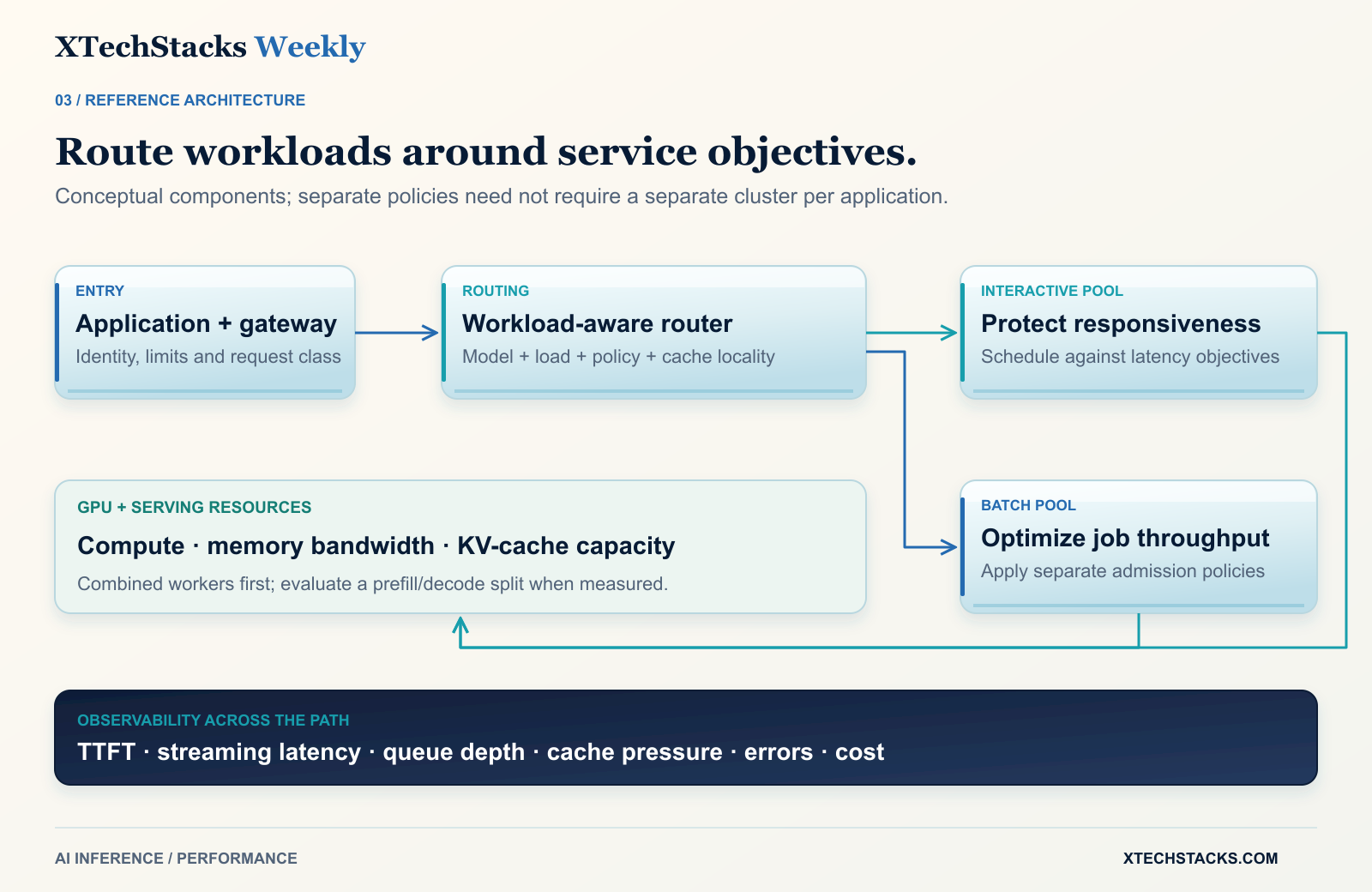
A practical enterprise serving architecture can retain the same general pattern regardless of whether the model runs on dedicated cloud GPUs, Kubernetes, or an on-premises cluster.
Application and AI gateway
Handles authentication, rate limits, request classification, and tenant-level policies.
Inference routing layer
Directs traffic to an appropriate serving pool based on model requirements, workload class, available capacity, and, where supported, cache locality.
Inference-serving engines
Run the models, schedule requests, manage KV cache, and generate tokens.
GPU infrastructure
Provides compute, high-bandwidth memory, and the network or interconnect resources needed by the architecture.
Observability and capacity management
Connects user-facing latency with request queues, prompt lengths, generated tokens, cache pressure, GPU telemetry, and cost.
One important design improvement is to distinguish workloads.
An interactive employee copilot may need low-latency responses.
A batch document-classification service may prioritize throughput.
A long-context research assistant may create substantial prefill pressure.
Putting every workload into the same shared inference pool without admission control or service-level differentiation can make capacity planning harder.
A better approach may separate latency-sensitive and batch traffic, or use scheduling and admission policies to protect critical requests.
This is not necessarily a case for separate GPU clusters for every application.
It is a case for explicit workload classes and measurable performance objectives.
What should enterprises do before buying more GPUs?
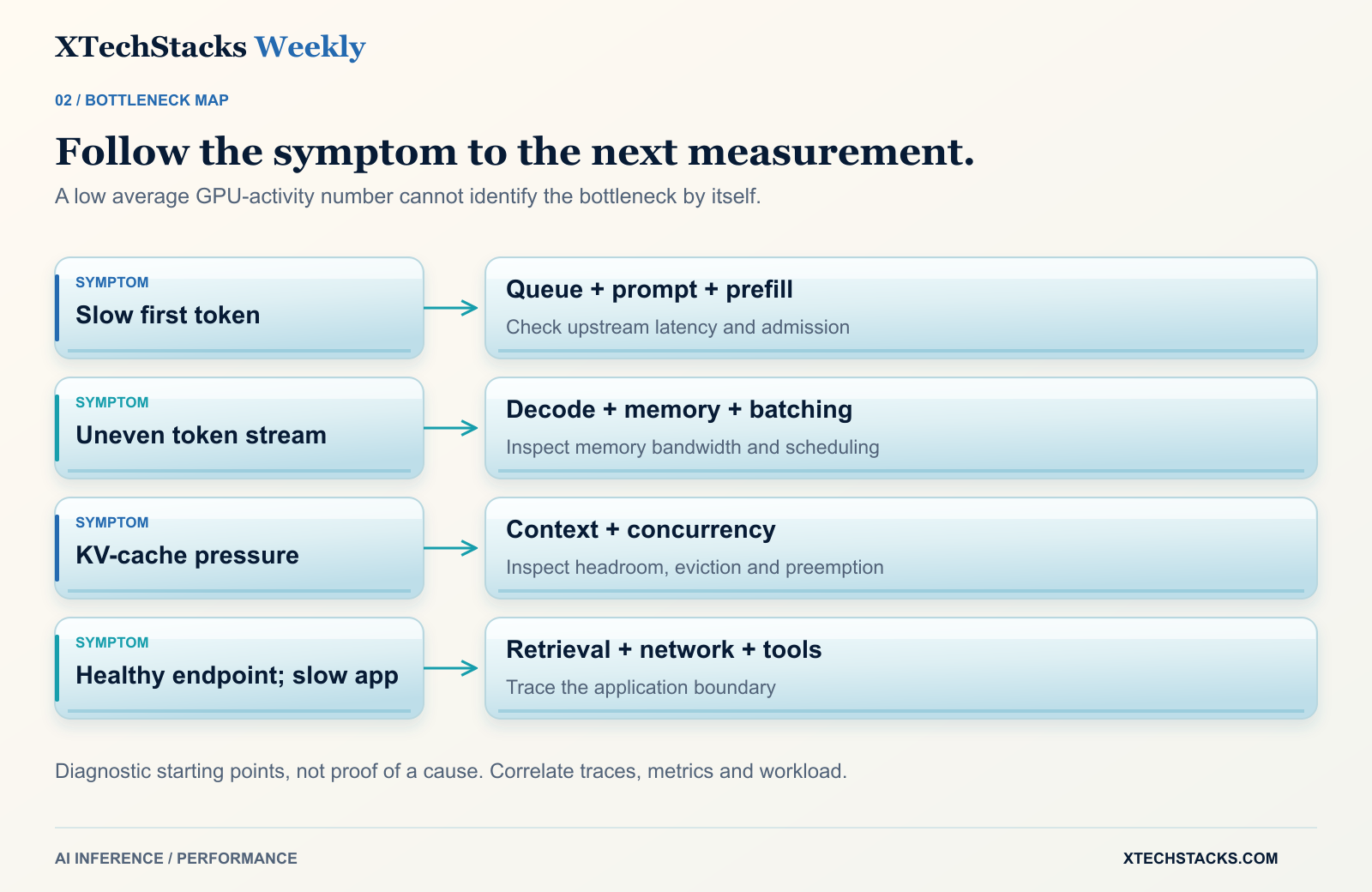
I would run an inference performance investigation using representative production traffic—appropriately anonymized or synthesized to protect sensitive data.
Begin by documenting the workload profile.
Capture the model and precision, GPU type, context-length distribution, output-length distribution, concurrency, arrival patterns, and current serving configuration.
Next, measure the system at different load levels.
Do not test only a single request or maximum synthetic concurrency.
Test ordinary traffic, realistic bursts, and sustained peak demand.
Then diagnose the bottleneck using the observed symptoms.
| Observed symptom | Investigate first |
|---|---|
| Slow first token, growing queue | Request admission, scheduler, available serving capacity |
| Slow first token, low queue | Prompt length, prefill, tokenization, upstream processing |
| Fast first token, slow streaming | Decode performance, memory bandwidth, batching |
| Latency spikes with long documents | Prefill interference, chunked prefill, workload separation |
| High KV-cache pressure | Context lengths, concurrency, cache allocation, preemption |
| Low cache benefit | Prefix reuse, prompt structure, cache residency and routing |
| Slow application, healthy inference endpoint | Retrieval, networking, middleware, tool calls, and application orchestration |
For each suspected bottleneck, change one meaningful variable at a time.
That may mean changing the batching configuration, enabling an appropriate cache feature, adjusting concurrency limits, testing another serving engine, or evaluating a different model size.
Record the before-and-after performance under comparable conditions.
Only after the system has been measured should the team decide whether additional GPU capacity is the correct investment.
The economic question: What are you actually paying for?
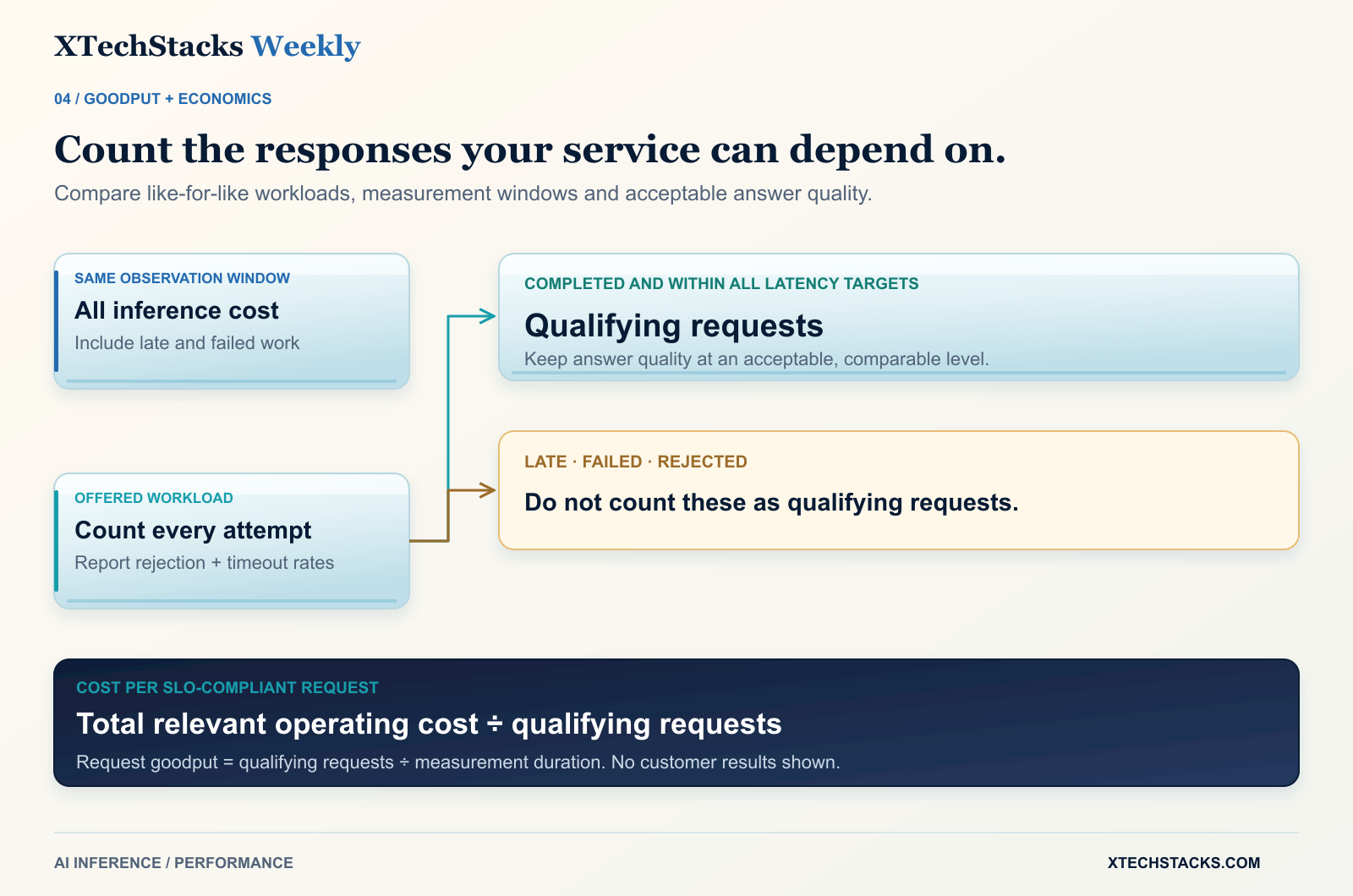
AI infrastructure spending is often discussed in terms of GPU-hour rates and cost per million tokens.
Those are useful financial measures.
But a business operating an AI application needs another view.
How much does it cost to deliver a response that meets the application's performance requirements?
A practical measure is:
Cost per SLO-compliant request = Total relevant inference operating cost ÷ Number of requests meeting the defined service-level objectives
The cost calculation may include GPU rental or amortization, serving infrastructure, networking, storage, observability, support, and operational overhead.
Use the same time window for the total cost and qualifying-request count. Costs incurred by failed or late requests stay in the numerator; those requests do not count in the denominator. Report offered load, rejection and timeout rates alongside goodput so admission control cannot hide unmet demand. Compare costs across equivalent workload mixes and acceptable answer quality.
This matters because a deployment producing more total tokens may not be economically superior if many user requests breach latency targets.
Likewise, a faster GPU might be more economical even at a higher hourly price if it delivers substantially more SLO-compliant requests.
But the reverse can also be true.
A less expensive GPU or smaller model may be perfectly adequate for a narrow enterprise workload.
There is no universal best GPU.
There is no universal best serving engine.
There is only a better or worse fit between the workload, its service requirements, and the infrastructure delivering it.
Where the business value appears
For SaaS companies, better inference performance can improve the responsiveness of AI-enabled product features while increasing the number of users served by existing infrastructure.
For manufacturing companies, inference optimization matters when deploying vision-language models, document analysis, and AI-assisted operational applications across plants or regional environments with constrained compute capacity.
For financial services, predictable latency and capacity isolation may be particularly important for time-sensitive internal applications, while security, audit, and data residency requirements influence deployment options.
For mid-market businesses, workload sizing can help avoid unnecessarily expensive GPU commitments or self-hosting decisions that create more operational complexity than value.
For consulting organizations, infrastructure benchmarking and serving optimization can become repeatable engineering engagements rather than one-time hardware procurement discussions.
The common problem is not simply expensive hardware.
It is the failure to connect infrastructure capacity to the actual needs of the AI application.
A practical 30-day approach
In the first week, establish a workload baseline.
Measure prompt lengths, output lengths, concurrency, TTFT, ITL, end-to-end latency, queue time, and cost.
In the second week, reproduce that workload in a controlled benchmarking environment.
Use a consistent model, hardware configuration, and load-generation method so the results can be compared. Record software versions, precision, warm-up, cold versus warm prefix-cache conditions, and arrival patterns. Include timeouts, rejected requests and failures rather than measuring completed requests alone.
In the third week, test a small number of targeted optimizations.
These might include chunked prefill settings, batching limits, prefix caching, alternative model configurations, or workload routing.
In the fourth week, compare performance and cost against the original baseline.
Document the maximum sustainable workload under the required latency targets, the operational trade-offs, and whether additional GPU capacity is necessary.
The deliverable should not simply be a faster benchmark.
It should be an evidence-backed infrastructure decision.
The real competitive advantage is efficient inference
The AI infrastructure market is moving quickly.
New GPUs offer greater computational capability.
Inference frameworks are becoming more sophisticated.
Distributed serving architectures are improving the way requests are scheduled, cached, and processed across hardware.
These developments are important.
But enterprise leaders should avoid confusing better hardware specifications with better application performance.
An inference platform must balance several competing objectives.
Low latency.
High throughput.
Efficient GPU memory usage.
Predictable performance under load.
Operational simplicity.
Acceptable infrastructure cost.
Optimizing one objective in isolation can make another worse.
The real engineering challenge is finding the right balance for the business.
Your GPU utilization dashboard tells you how busy the hardware appears to be.
Your inference performance metrics tell you what users experience.
Your cost per SLO-compliant request tells you whether the architecture is economically sustainable.
Enterprises that understand all three will be better positioned to scale AI without assuming that every performance problem requires another GPU.
A question for technology leaders
When AI response times deteriorate in your environment, what does your team investigate first: GPU utilization, application latency, request queues, or the behavior of the inference engine itself?
I'd be interested in hearing which inference bottlenecks have been most difficult to diagnose in production.
For related guidance, explore our AI platform engineering approach and guide to operating LLM applications.
— XTechStacks
Technology · AI · Strategy · Impact
References and further reading
- NVIDIA — How to Size GPUs for AI Inference and TCO Without Overspending, September 1, 2026.
- Microsoft Research — Reproducible LLM Inference Benchmarking, October 2026.
- NVIDIA — Benchmarking LLM Inference at Scale with AIPerf, September 18, 2026.
- vLLM — Production Metrics.
- vLLM — Optimization and Tuning.
- NVIDIA Dynamo — Disaggregated Serving.
- Red Hat — Five Steps to Triage vLLM Performance, March 9, 2026.
The opening SaaS scenario is illustrative. No performance gain is presented as an XTechStacks customer result. Framework behavior depends on the version and deployment configuration.